Quality Control in Statistical Analyses

statistics

Experienced statisticians and data analysts are familiar with stories where a coding error has led to an entire conclusion changing, even leading to a retraction. It’s the sort of stuff that keeps people up at night.

Author

Zad Rafi

Published

June 13, 2020

Keywords

statistical reporting, statistics, accuracy, data science

Experienced statisticians and data analysts are familiar with stories where a coding error has led to an entire conclusion changing, or even a retraction.[@aboumatarNoticeRetractionAboumatar2019] It’s the sort of stuff that keeps people up at night. Unfortunately, not many of us think about these sorts of scenarios until we realize it’s very possible that it could happen to any of us.

To me, it seems that many of these issues could be avoided by having a principled data management and statistical workflow, and making it as transparent, open, and reproducible as possible. I’d like to quickly go over a few things that I’ve found helpful over the years, and I’ll first start with data management and data entry and then move onto analysis workflows. I largely consider this to be a living document, and I’m sure many people who will read this will have far better suggestions, so please leave them down below in the comments!

Before I go on, I want to emphasize that backing up your data, scripts, and using version control is extremely important. There is no debate about this. It’s necessary so that other collaborators/colleagues can inspect your work and catch potential mistakes or see overall progress, but more importantly, it will prevent you from losing your data in a disaster, and it’ll help you catch your own mistakes, since you’ll be the most familiar with the data and scripts.

1 Data Entry & Management

A nice paper that I’d like to review is the one by Broman & Woo, 2018 on how to manage your data when working with spreadsheets.[@bromanDataOrganizationSpreadsheets2018] The sad reality is that even though spreadsheets like Microsoft Excel or Google Sheets are available everywhere, and easy to use, there are many risks when working with spreadsheets, just ask any statistician who works in genetics or any bioinformatician.[@ziemannGeneNameErrors2016]

One of the most fatal errors occurred recently when a group of researchers lost thousands of documented COVID cases because they entered data for each case as a column instead of a row, and Excel has a limit on how many columns and rows it can handle (1,048,576 rows and 16,384 columns, according to Microsoft), as a result, most of these cases were lost, resulting in an enormous waste of resources due to a careless and ignorant mistake, highlighting the dangers of recklessly inputting data and conducting statistical analyses. There is no doubt that reviewing principles of good data management and workflow are essential to any data analyst. I’d like to touch on some of the most important points of Broman & Woo, 2018 paper before moving onto some other “principles” I’d like to share:

1.1 General Principle: Be Consistent With Everything

When labeling missing values (NA, N/A, etc.):
- Good: Choose one method (NA, N/A, etc.) and stick with it.
- Bad: Leaving cells empty to indicate missingness.

When labeling response variables:
- Good: If you label a response variable consistently, for example, fat-free-mass in every instance to refer to the same variable.
- Bad: If you label a response variable fat-free-mass in one script/sheet, and ffm/fat_free_mass in another.

When formatting variable predictor names:
- Good: predictor_1_week12, predictor_2_week12, response_variable_week12. This is consistent, with the order of the names, and dates/weeks, so it is easier to organize, inspect, and clean. Same thing applies to labeling response variables and pretty much all variables.
- Bad: When you label one variable week12_predictor_1, the next predictor_2_week12, and the last, 12_week_response. Just no.

When formatting dates:
- Good: Use one format, YYYY-MM-DD, consistently.
- Bad: Everything else.

When filling out cells:
- Good: One cell = one thing. No more, no less.
- Bad: One cell = multiple entries or no entries at all.

When keeping track of the data:
- Good: Create a comprehensive data dictionary so anyone can look at it and understand the spreadsheets/dataframes/variables.
- Bad: Expecting yourself and others to figure it out based on the variable names that you thought were brilliant.

When using Excel or Google Sheet’s shiny features:
- Good: Avoid using any of them, any formulas, highlighting, italicizing, bolding, etc.
- Bad: If you’re the type of person to create charts in Excel.

Planning for disasters:
- Good: Always, always, backup your files, save them in .txt files. Keep backups of those. And most importantly, use version control!
- Bad: You don’t really plan for disasters and go with the flow.

Last but not least, when entering cases:
- Good: Rows are for cases and observations, and columns are for variables and characteristics. Please do not switch these up!
- Bad: Using them interchangeably.

2 Setting Up a Principled Statistical Workflow

Here’s what I’ve been doing for many years and what seems to work for me (none of these ideas are originally mine, and I actually picked them up over the years from others’ advice, which will be linked below).

2.1 Setting up the Project Folder

When setting up a folder specific for a project (if you’re not doing this, you absolutely need to), first, I will create a folder with the title of my project, and usually have an RStudio project set up in there.

Disclaimer: while much of this advice will be familiar and easy to understand for those who use R, I think the general principles are widely applicable, especially for those who use scripts in their statistical software).

This folder will contain many other folders (more on that below), so the structure will end up being a bit complex.

workflow

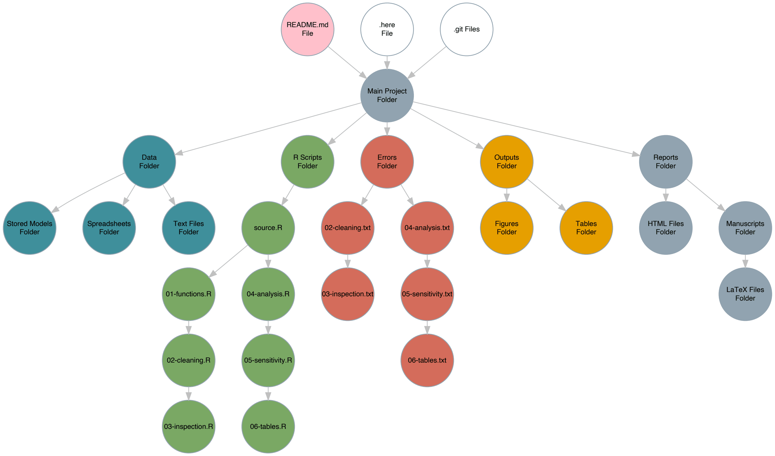
It may be a bit difficult to read the words within the circles, but clicking on the diagram should enlargen it and allow you to zoom in, giving you a sense of how I organize all these scripts and files.

If this ends up confusing you, you can just scroll all the way down to see an image of what the folder structure looks like.

Instead of constantly changing the working directory to each subfolder when I need to do something inside that subfolder for a particular project or analysis, I set the project folder as the working directory only once, and then run the following:

Code

# Very seriously consider installing the `here` package

# https://cran.r-project.org/package=here

library("here") 

# This and the scripts below take
# the directory used and set it as the top

set_here() 

here()

This not only sets the working directory, but gives you far more control over how you can save your files from any place within the hierarchical folder structure. It will create a file called .here inside the Main Project folder, which will indicate that this is the top level of the hierarchy.

Then, I will usually have created a README.Rmd file in the Main Project folder with updates on what I’ve done and what I still need to work on, so I will remember and so my collaborators can see it too (when it has been pushed to GitHub or other version control repos).

Next, I’ll set up a Data folder inside the Main Project folder. This is where all my data/spreadsheets/.txt files and data dictionaries will go. The original data files will stay inside this folder, while I create two other subsubfolders inside this Data folder called Transformed and Models. In Transformed, I will typically save .rds files that were a result of cleaning and transforming the data, including imputing missing data. I will touch more on exactly how I do that later below. A Models subfolder will obviously store fitted models and any validation/sensitivity analyses of those models.[@morrisChoosingSensitivityAnalyses2014]

Now, back to the Main Project folder, I’ll set up another folder within it called R. This will be where all of my .R scripts/files live. I will number them sequentially along with a title for a specific purpose, like so

main.R
01-functions.R
02-cleaning.R
03-inspection.R
04-analysis.R
04.5-validation.R
05-sensitivity.R
06-tables.R

2.2 Setting up the Functions Script

All potential R packages and custom functions that I need will belong in 01-functions.R. This .R file will only serve this purpose and nothing else. As you’ve guessed by now, the other .R files will be doing the same, they have very specific purposes and are organized to reflect this.

An example of the first script can be found below.

Code

# Necessary Packages ------------------------------------

req_packs <- c("rms", "concurve", "mice", 
               "tidyverse", "parallel", 
               "bayesplot", "projpred", 
               "Hmisc", "loo", "rstan", "here",
               "tryCatchLog", "futile.logger", 
               "patchwork", "corrplot", "beepr", 
               "summarytools", "broom", "wakefield", 
               "boot", "mfp", "knitr", "flextable", 
               "MASS", "lme4", "brms", "miceMNAR")

# Load all packages at once

lapply(req_packs, library, 
       character.only = TRUE)

# Loggings messages 
options(keep.source = TRUE)        
options("tryCatchLog.write.error.dump.file" = TRUE) 

# Set seed for random number generator

RNGkind(kind = "L'Ecuyer-CMRG")
set.seed(1031) # My birthday

# RStan Settings  -------------------------------------

theme_set(theme_bw())
color_scheme_set("red")
rstan_options(auto_write = TRUE)
options(mc.cores = 4)

has_build_tools(debug = TRUE)

# Stan Settings  ---------------------------------------

dotR <- file.path(Sys.getenv("HOME"), ".R")
if (!file.exists(dotR)) dir.create(dotR)
M <- file.path(dotR, "Makevars")
if (!file.exists(M)) file.create(M)
cat("\nCXX14FLAGS=-O3 -march=native -mtune=native -fPIC",
  "CXX14=g++", 
  file = M, sep = "\n", append = TRUE)

The script above loads all the necessary R packages each time it is called, along with the specified functions, so most of the other .R files will depend upon this one.

However, I will not be running each of these .R files/scripts individually, line by line, or by selecting all the lines in an .R file and running the script.

Instead, after I’ve created all these files (figuring out what I need to do carefully and writing it down and annotating it), every single .R file except for main.R will have the following script, which I will explain later below (or some iteration of this script to match the name of the file) at the beginning:

2.3 Setting up the Error Catching Script

Code

library("here")

set_here()

source(here("R", "01-functions.R"))

library(futile.logger)
library(tryCatchLog)

# Keeps source code file name and line number tracking
options(keep.source = TRUE)        
options("tryCatchLog.write.error.dump.file" = TRUE) 

# Logs messages into a file 
flog.appender(appender.file("my_app.log"))  
flog.threshold(INFO)   

# Function that catches any messages
tryCatchLog(source("script.R"))

You’ll notice several things. First, I’m once again calling the here package and telling it that I’m working within this folder (R), and then I’m calling the 01-functions.R file by using the source() function, but also notice how the source() function is followed by a here() function/argument. This here() function allows you to fully control files in a specific folder from anywhere else, without having to actually be in that folder. So, suppose I was in the Main Project -> Data -> Models folder and I was saving my work there (in the Models folder), which is pretty far from the R folder, I can still, using functions like source(), save(), etc., call or manipulate files from a totally different folder by specifying the hierarchy using here(). This can also be done in other ways, but those are far more cumbersome, and not flexible.

This is how I always call the necessary packages and functions I need from every .R script, simply by using the source() function and using here() to direct it to the 01-functions.R file in the R folder. Now let’s look at the next few lines.

Code

flog.appender(appender.file("script.log"))
flog.threshold(INFO)    

tryCatchLog(source("script.R"))

This script is designed to catch any warnings that occur inside the .R script and save them to a .log file in another subfolder within the R folder called Errors. So here’s an example of a full script for a mix of data generation and inspection, so that you can see it in action.

2.4 Example of Data Loading & Inspection

Code

library("here")

set_here()

source(here("R", "01-functions.R")) # Loads all R functions

# First we need some data

RNGkind(kind = "L'Ecuyer-CMRG")
set.seed(1031) # My birthday

# Suppose you wanted to simulate a clinical trial
library("simstudy")  

# Simulating a Clinical Trial --------------------------

def <- defData(varname = "male", dist = "binary", 
               formula = .5 , id="cid")
def <- defData(def, varname = "over65", 
               dist = "binary",
               formula = "-1.7 + .8 * male", 
               link = "logit")
def <- defData(def,varname = "baseDBP", 
               dist = "normal",
                 formula = 70, variance = 40)
def <- defData(def, varname = "age", 
               dist = "normal", 
               formula = 10, 
               variance = 2)
def <- defData(def, varname = "visits", 
               dist = "poisson", 
    formula = "1.5 - 0.2 * age + 0.5 * male", 
    link = "log")
def <- defData(def, varname = "weight", 
               dist = "normal",
                 formula = 60, variance = 10)
dtstudy <- genData(500, def)
study <- trtAssign(dtstudy, nTrt = 2, 
                   balanced = FALSE, grpName = "rxGrp")
study <-  as.data.frame(study)
study$iq <- iq <- wakefield::iq(500)
study$height <- height <- wakefield::height(500)
study$income <- income <- wakefield::income(500, 
                              digits = 2, name = "Income")
study$SAT_score <- wakefield::sat(500, mean = 1500, 
                 sd = 100, min = 0, max = 2400, 
                 digits = 0, name = "SAT")
study$visits <- as.numeric(study$visits)
# Add noisy predictors
study[, 11:20] <- lapply(1:10, FUN = function(i) 
                         (rnorm(n = 500, 
                                mean = 1, sd = 2)))
varname <- sprintf("x%d", (11:20))
colnames(study)[11:20] <- varname

study1 <- trtAssign(dtstudy, n = 2, balanced = TRUE, 
                    strata = c("male", "over65"), 
    grpName = "rxGrp")

study1

# Inspecting Data  -------------------------------------

summarytools::view(dfSummary(study))

study$over65 <- as.factor(study$over65)
study$male <- as.factor(study$male)
study$rxGrp <- as.factor(study$rxGrp)

study_formula <- as.formula(baseDBP ~ .)

plot(spearman2(study_formula, study))
abline(v = 0)

x_1 <- model.matrix(~ ., data = study)[, -1]

# Initial Data Analysis  ------------------------------

(cormatrix <- (cor(x_1)))

col <- colorRampPalette(c("#BB4444", "#EE9988", 
                          "#FFFFFF", 
                          "#77AADD", "#4477AA"))

corrplot(cormatrix, method = "color", 
         col = col(200), 
         tl.col = "black", tl.cex = 0.40,
         addCoef.col = "black", number.cex = .35)


clus1 <- varclus(x_1, similarity = "h")
clus2 <- varclus(x_1, similarity = "s")
clus3 <- varclus(x_1, similarity = "p")

plot(clus1, ylab = "Hoeffing's D statistic", 
     lwd = 2.5, lty = 1, cex = 0.75)
title("Hierarchical Cluster Analysis")


plot(clus2, lwd = 2.5, lty = 1, cex = 0.75)
plot(clus3, lwd = 2.5, lty = 1, cex = 0.75)

Pre <- names(study)
(fmla <- as.formula(paste("~", 
                          paste(Pre, 
                                collapse = "+"))))

# Redundancy analysis 

redun <- redun(fmla,
  data = study,
  r2 = 0.90, type = "ordinary", allcat = FALSE,
  tlinear = FALSE, iterms = FALSE, pr = TRUE)

The above script simulated some fake data for a hypothetical clinical trial (usually we use this first script to load data from a .csv or .txt file) and then we used several functions to inspect the dataframe for the structure and distributions of the variables and missing data, etc. We also attempted to properly code the variables. Now, in order to capture any possible errors, we will have to run this entire script from another R script instead of running it line by line or selecting all the code and running it.

We will do this from a Main source script, which will allow us to use the tryCatchLog() function.

2.5 Example of the Main Source Script

Code

library("here") 
library("tryCatchLog")
library("futile.logger")

set_here() # Load and set here

here() # Call here

options(keep.source = TRUE)        
options("tryCatchLog.write.error.dump.file" = TRUE) 

# Script loads all necessary functions
flog.appender(appender.file(
  here("Errors", "01-functions.log")))
tryCatchLog(source(here("R", "01-functions.R"))) 

# Line script to clean the data
flog.appender(appender.file(
  here("Errors", "02-cleaning.log")))
tryCatchLog(source(here("R", "02-cleaning.R"))) 

# Line script below to inspect the data
flog.appender(appender.file(
  here("Errors", "03-inspection.log")))
tryCatchLog(source(here("R", "03-inspection.R")))  

# Load saved objects from cleanings
flog.appender(appender.file(
  here("Errors", "03.5-load_data.log")))
tryCatchLog(source(here("R", "03.5-load_data.R"))) 

# Main analysis script
flog.appender(appender.file(
  here("Errors", "04-analysis.log")))
tryCatchLog(source(here("R", "04-analysis.R")))  

# Below is the validation of main analysis results 
flog.appender(appender.file(
  here("Errors", "04.5-validation.log")))
tryCatchLog(source(here("R", "04.5-validation.R"))) 

# Test the sensitivity of the results by
# varying assumptions/multiple parameters
flog.appender(appender.file(
  here("Errors", "05-sensitivity.log")))
tryCatchLog(source(here("R", "05-sensitivity.R"))) 

# Generate tables and figures of all your results 
flog.appender(appender.file(
  here("Errors", "06-tables.log")))
tryCatchLog(source(here("R", "06-tables.R"))) 

# Export these into actual files that can be
# inserted into papers, reports, etc.
flog.appender(appender.file(
  here("Errors", "07-export.log")))
tryCatchLog(source(here("R", "07-export.R")))

If anything went wrong during the simulations and their inspections in the first script from above, it would have been captured by the error-catching scripts that we have set up, which would be placed within a .log file in the Errors folder, which is inside the R folder.

2.6 Setting the Seed

Also, note that we have set the seed using a specific random number generator algorithm. This is not that important, however, it is important to correctly set the seed for reproducing any random numbers generated. This requires even more careful thought when running a simulation study, in which the states of the simulation need to be saved for a particular repetition, and so that streams do not overlap.[@morrisUsingSimulationStudies2019]

I will admit that the error script is not perfect at capturing warnings, but for most things, if something wrong occurs when a script is run, the function tryCatchLog() and its .log file usually catches the warning, so I would know that something went wrong and what specifically.

However, some may be skeptical of this approach and ask why I need to catch these errors and save them if I ran the scripts? Why not just scroll up and look at the console to see the errors or warnings?

Many reasons:

Suppose the analyses take a very long time, and are computationally intensive, and R/RStudio crashes, you may not be able to figure out what went wrong.
Suppose the analysis completed but because there was so much occurring in the console (for example, sampling from a posterior) that you missed the warnings/errors and got results that you don’t know have issues.

Thus, having this system set up to catch errors in every script also helps us automate the entire workflow once we’ve carefully set it up. After each .R script has one of these message-catching scripts, we can run our entire analysis from start to finish from main.R with one command. This not only makes your workspace organized, but also makes it easier for others to reproduce your work if you share your files and folders via a repository.

So, now the Error folder will contain .txt files with any warning messages or errors.

Typically, when I’m setting up a new project, I will also add a few other folders such as an Outputs folder, where I will save tables and graphs, and a Report folder, where I might be working on a manuscript.

Now that I’ve mentioned my hierarchy and how I catch errors, I can mention some other things that I believe are absolutely heinous practices.

Many people often will run an entire analysis and have several objects/vectors stored in their Global Environment in R and RStudio. Suppose they’re taking a break, finished with the analysis, turning off the computer, or stepping away for whatever reason, what they’ll typically do is click the save button on the top right pane and “Save the workspace image”. Indeed, if they don’t do that themselves, the IDE RStudio will explicitly ask them if they wish to save their workspace image.

This is a horrific practice and you should never do this because it can lead to several problems such as:

having several saved objects and packages conflict with one another once they’re all loaded together at once
having giant workspace images, that will probably cause R, and especially RStudio to constantly crash
not allowing you to load very specific objects that you need at a time while leaving everything else

I would say that it is a good idea to never save the workspace image, ever. It is also quite easy to turn off. Simply go the RStudio menu and click Preferences, and in the General section, you will see the following options:

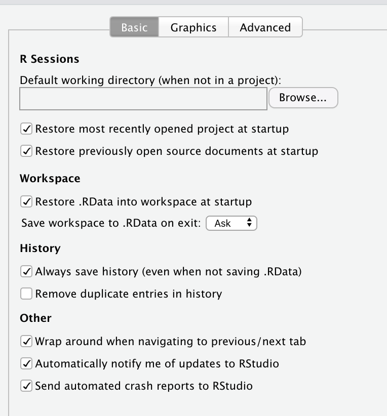
It is essential to uncheck everything under R Sessions, Workspace, and History, so that you do not set your self up for a future disaster.

Instead of using these convenient but highly problematic options, always use the saveRDS() base R function, where the first argument is the object in your environment that you want to save, and the second argument is the path where you want to save it, which of course should be using the here() function.

Now suppose I decided to use multiple imputation because I had a dataset with many missing values, and suppose I had a grasp of the missing data mechanism, and so I used something like the not-at-random fully conditional specification approach (NARFCS)[@tompsettUseNotatrandomFully2018] to attempt to handle data that I believe to be missing not at random (MNAR), and I wanted to save the imputed dataset, and only load the imputed dataset next time. This is how I would do it (in the vaguest way possible). First, I’ll start with the dataset that we generated above and generate missing values via different missing data mechanisms using the ampute() function from the mice package.[@buurenMiceMultivariateImputation2011]

Important: This is all assuming that one has carefully constructed an imputation model, and that multiple imputation is the most appropriate solution. As many others have pointed out, simply running a script like mice(data) in R without careful thought to the imputation model, is a very, very bad idea. Missing data is an extremely complex topic and I recommend everyone carefully read the works[@buurenFlexibleImputationMissing2018] of missing data researchers such as:

2.7 Example of a Multiple Imputation Script

Code

source(here("R", "01-functions.R"))

library("beepr")

# Package that uses multiple imputation
# by chained equations

library("mice") 
     

# Generate Missing Data  --------------------------------

study_mnar <- ampute(data = study[, 5:10], 
                     prop = 0.65, mech = "MNAR")
mnar_patterns <- study_mnar$patterns
mnar_weight <- study_mnar$weight
study_mnar_rerun <- ampute(data = study[, 5:10], 
                           prop = 0.5, 
                           mech = "MNAR", 
                           patterns = mnar_patterns,
                           weights = mnar_weight)
study_mar <- ampute(data = study[, 2:4], prop = 0.5, 
                    mech = "MAR")
mar_patterns <- study_mar$patterns
mar_weight <- study_mar$weight
study_mar_rerun <- ampute(data = study[, 2:4], 
                          prop = 0.5, 
                          mech = "MAR", 
                          patterns = mar_patterns,
                          weights = mar_weight)

study_mar_rerun[[11]]$over65 %>% 
  as.factor()
study_mar_rerun[[11]]$male %>% 
  as.factor()
study_mar_rerun[[11]]$rxGrp %>% 
  as.factor()

df <- study_mnar_rerun$amp
df2 <- study_mar_rerun$amp

# Inspect Data

str(df) # Inspect data frame
summary(df) # High level summary of dataframe
sum(is.na(df)) # Look at missing values etc.
colSums(is.na(df))
summarytools::view(dfSummary(df)) 

str(df2) # Inspect data frame
summary(df2) # High level summary of dataframe
sum(is.na(df2)) # Look at missing values etc.
colSums(is.na(df2))
summarytools::view(dfSummary(df2)) 

# Prepare Data for Imputation -------------------------

temp <- df
temp2 <- df2

missing_plot(temp)

missing_plot(temp2)

# Set-up predictor matrix

predMatrix <- make.predictorMatrix(temp)
predMatrix2 <- make.predictorMatrix(temp2)

# Set-up predictor matrix for unidentifiable part:
predSens <- matrix(rep(0, 6), ncol = 6, nrow = 6)
colnames(predSens) <- paste(":", names(temp), sep = "")
rownames(predSens) <- names(temp)

# Set-up list with sensitivity parameter values

pSens <- rep(list(list("")), ncol(temp))
names(pSens) <- names(temp)
pSens[["rxGrp"]] <- list(-.4)
pSens[["baseDBP"]] <- list(-.4)
pSens[["male"]] <- list(-.4)
pSens[["over65"]] <- list(-.2)

# MICE RI Imputation  ----------------------------------

z1 <- parlmice(data = temp, method = "ri",
              predictorMatrix = predMatrix,
              m = 8, maxit = 1, 
              cluster.seed = 1031, n.core = 4, 
              n.imp.core = 2, cl.type = "FORK", 
              ridge = 1e-04, remove.collinear = TRUE, 
              remove.constant = FALSE, allow.na = TRUE) 

z2 <- parlmice(data = temp2, method = "pmm",
              predictorMatrix = predMatrix2,
              m = 8, maxit = 1, 
              cluster.seed = 1031, n.core = 4, 
              ridge = 1e-04, remove.collinear = TRUE, 
              n.imp.core = 2, cl.type = "FORK") 

zfinal <- cbind(z1, z2)

# Heckman Imputation  ----------------------------------

study$baseDBP <- temp$baseDBP
JointModelEq<-generate_JointModelEq(data=temp, 
                                    varMNAR="baseDBP")
JointModelEq[,"baseDBP_var_sel"] <- c(0,1,1,1,1,1)
JointModelEq[,"baseDBP_var_out"] <- c(0,1,1,1,1,1)

arg <- MNARargument(data = temp, varMNAR = "baseDBP", 
                    JointModelEq = JointModelEq)

arg$method["age"] <- "ri"
arg$method["visits"] <- "ri"
arg$method["weight"] <- "ri"
arg$method["iq"] <- "ri"
arg$method["height"] <- "ri"

imp1 <- parlmice(data = arg$data_mod,
                  method = arg$method,
                  predictorMatrix = arg$predictorMatrix,
                  JointModelEq = arg$JointModelEq,
                  control = arg$control,
                  maxit = 1, m = 8,
                  cluster.seed = 1031, n.core = 4, 
                  n.imp.core = 2, cl.type = "FORK")

analysis1 <- with(zfinal, glm(baseDBP ~ age + visits + weight + iq + height + rxGrp + male + over65))
result1 <- pool(analysis1)
summary(result1)

z2 <- parlmice(data = temp2, method = "pmm",
              predictorMatrix = predMatrix2,
              m = 8, maxit = 1, 
              cluster.seed = 1031, n.core = 4, 
              n.imp.core = 2, cl.type = "FORK") 

heckman <- cbind(imp1, z2)

beep(3) # I will touch on this function below.

saveRDS(zfinal, here("Main Project", "Data", 
                     "zfinal.rds"))

Here is the workflow truly showing its advantages, saveRDS() is saving a very specific object (zfinal, the imputed dataset) into the Data folder by using the hierarchical structure of the folder which can easily be navigated using here(). Notice how to save something and use here() to specify the location, the first argument is Main Project, followed by Data, and then comes the object name (zfinal.rds).

Now I have saved my imputed dataset as an object called zfinal.rds and it is saved in the Data folder even though I am hypothetically working from the R folder.

Also notice that I use the beep() function from the beepr R package, which can be quite handy in letting you know if a particular script or analysis is done.

Next time, if I cleared my entire global environment and wanted to only load the imputed dataset, I would simply have to just click on the zfinal.rds file in the Data folder and it would load into the environment or I could use the following command,

2.8 Saving and Reading Data Carefully

Code

# The function readRDS() and saveRDS()
# are possibly the most important base R functions

zfinal <- readRDS("zfinal.rds", 
             here("Main Project", "Data", 
                  "zfinal.rds"))

This gives us full control over the environment, and it’s also why I encourage people to turn off the automatic prompt to save the workspace that RStudio gives you by default (I am certain even Hadley Wickham has said the same on multiple occasions).

So if I now wanted to include the imputed dataset into one of my .R scripts that I am trying to automate with one command, whether for reproducibility, or speed, etc., I could do it with absolute control.

This is also how I save my models and how I validate them, which is especially handy because running those can also take an excruciatingly long time.

Here’s an example of a script that would be in the 04-analysis.R script, I’m leaving out the warning-catching script now to avoid making this too long. I don’t need to load the brms package because I’m already calling it from the first .R script, 01-functions.R (but I’m just showing it for now to avoid confusion), and then I am saving it in the Models folder which is found in the Data folder. And again, the beep() function would let me know when the script is over, and scripts like this can often take very long, due to the computational intensity.

The script below is an analysis script whose results we plan on saving once completed. Due to the arguments I have set (iterations, warmups, chains, and using an imputed dataset), it can often take a long time before it is finished, and if I did happen to do other tasks while I was waiting on that, the output would automatically save to the Models folder via saveRDS(), and I would also receive a notification via the beep() function, preventing me from wasting any time.

2.9 Example Modeling Script

Code

# Calling all packages, please report for duty

source(here("R", "01-functions.R")) 

library("brms") 

# This is a script I used previously
# where I used Bayes for regularization  
# Although these are all generic options 

# Prior Information  --------------------------------

sample_z <- complete(zfinal, 1)

n_1 <- nrow(sample_z) # of observations

k_1 <- (ncol(sample_z) - 1) # of predictors

p0_1 <- 2 # Prior for the number of relevant variables

tau0_1 <- p0_1 / (k_1 - p0_1) * 1 / sqrt(n_1) # tau scale

# Regularized horseshoe prior
hs_prior <- set_prior("horseshoe(scale_global = tau0_1, 
                      scale_slab = 1)", class = "b")

library("future")
plan(multiprocess)

# Regularized Bayesian quantile
# regression using regularized horseshoe prior
brms::brm_multiple(
  bf(baseDBP ~ age + visits + weight + iq + height + rxGrp + male + over65, 
     quantile = 0.50),
     data = zfinal, prior = hs_prior, 
     family = asym_laplace(), sample_prior = TRUE,
     seed = 1031, future = F,
     iter = 1000, warmup = 500, chains = 4, 
     cores = 4, thin = 1, combine = TRUE, 
     control = list(max_treedepth = 10, 
                    adapt_delta = 0.80)) -> pen_model_1

# Principled way of saving results
saveRDS(pen_model_1,   
        here("Main Project", "Data", "Models", 
             "pen_model_1.rds")) 

beep(3)

So I’ve saved the full contents of the fitted model (pen_model_1), which are usually several gigabytes large in size, within the Models folder. Once again, notice how the here() function allows you to work from a subfolder like R, which is inside the Main Project folder, and allows you to specify the hierarchy, and where you are within it, and save to whichever folder you wish, in this case Models, which is inside of Data. Now, I will typically conduct model checks and make sure it is performing well, and not misspecified,

Code

source(here("R", "01-functions.R")) 

# Inspect RHat values ---------------------------
 
rhats_1 <- pen_model_1$rhats

rhats_1_df <- (rhats_1 <= 1.1)
((as.numeric(table(rhats_1_df)) / 
    (nrow(rhats_1_df) * ncol(rhats_1_df)) * 100))

rhats_1_vec <- as.numeric(unlist(c(
  rhats_1[, 1:ncol(rhats_1)])))

pdf(here("Outputs", "Figures", "Diagnostics", 
         "OUTCOME_COMP_rhat.pdf"))
mcmc_rhat_hist(rhats_1_vec) +
  ggtitle("Model 1 Chain Convergence")
dev.off()

# Inspect Effective Sample Size ----------------------

mcmc_neff_hist(rhats_1_vec) +
  ggtitle("Effective Sample Size")

# Inspect Divergences ---------------------------

pdf(here("Outputs", "Figures", 
         "Diagnostics", "OUTCOME_1.pdf"))
mcmc_nuts_divergence(nuts_params(pen_model_1), 
                     log_posterior(pen_model_1))
dev.off()

# Examine Residual Plots ----------------------------

df_resid_stan_1 <- data.frame(fitted(pen_model_1)[, 1], 
                              residuals(pen_model_1)[, 1])

pdf(here("Outputs", "Figures", 
         "Diagnostics", "OUTCOME_1.pdf"))
ggplot(df_resid_stan_1, 
       aes(sample = residuals(pen_model_1)[, 1])) +
  geom_qq() +
  geom_qq_line() +
  ggtitle("Model 1 Residuals")
dev.off()

(sum1 <- (posterior_summary(pen_model_1))[2:8, ])

mcmc_intervals(pen_model_1, point_est = "median", 
               prob = 0.95, prob_outer = 0, 
               pars = parnames(pen_model_1)) +
  ggplot2::scale_y_discrete() +
  theme(axis.text=element_text(size=13),
        axis.title=element_text(size=13),
        plot.title = element_text(size=15, 
                                  face = "bold")) +
  annotate("rect",
    xmin = -0.05, xmax = 0.05, ymin = 0, ymax = 7,
    fill = "darkred", alpha = 0.075) +
  annotate("segment",
    x = -0.05, xend = -0.05, y = 0, yend = 7,
    colour = "#990000", alpha = 0.4, 
    size = .75, linetype = 3) +
  annotate("segment",
    x = 0.05, xend = 0.05, y = 0, yend = 7,
    colour = "#990000", alpha = 0.4, 
    size = .75, linetype = 3) + 
  ggtitle("Change in Outcome 1")
dev.off()

pdf(here("Outputs", "Figures", "OUTCOME_1.pdf"))
mcmc_hist(pen_model_1)

# Posterior Predictive Checks
 
pdf(here("Outputs", "Figures", "Diagnostics", 
         "OUTCOME_1check.pdf"))
pp_check(pen_model_1, nsamples = 250) + 
  ggtitle("Posterior Predictive Check: Model 1")
dev.off()

# Shows dens_overlay plot by default

bayes_rsq1 <- bayes_R2(pen_model_1)

bayes_rsq1 <- print(median(bayes_rsq1))

write.csv(sum1, here("Outputs", "Tables", 
                     "OUTCOME_1.csv"))

Once I have fit my model and done some initial checks, I usually conduct some more thorough checks using k-fold cross-validation or nested cross-validation, or bootstrap optimism.

A script of this can be found below.

Code

source(here("R", "01-functions.R"))

# 10-Fold Cross-Validations -------------------------

kfold_1 <- kfold(pen_model_1, K = 10, 
                 save_fits = TRUE, cores = 4)
saveRDS(kfold_1, here("Data", "Models", 
                      "Validation", "kfold_1.rds"))
kfp_1 <- kfold_predict(kfold_1)
saveRDS(kfp_1, here("Data", "Models", 
                    "Validation", "kfp_1.rds"))
kfold_rmse(y = kfp_1$y, 
           yrep = kfp_1$yrep, 
           type = "rmse", 
           reps = 5000, 
cores = 4)[[2]][["t"]]) -> kfold_rmse_1

kfold_rmse_1 <- median(kfold_rmse_1)

saveRDS(kfold_rmse_1, 
        here("Data", "Models", 
             "Validation", "kfold_rmse_1.rds"))

Once I’ve written all my analysis and validation scripts, I’ll typically create a subfolder in the Outputs folder called Figures and Tables and save them appropriately with the help here().

2.10 Example Table Script

Code

source(here("R", "01-functions.R"))

# Read in Validation Objects ------------------------

kfold_1 <- readRDS("kfold_1.rds", 
                   here("Main Project", "Data", 
                        "Models", "Validation", 
                        "kfold_1.rds"))
kfold_2 <- readRDS("kfold_1.rds", 
                   here("Main Project", "Data", 
                        "Models", "Validation", 
                        "kfold_2.rds"))
kfp_1 <- readRDS("kfp_1.rds", 
                 here("Main Project", "Data", 
                      "Models", "Validation", 
                      "kfp_1.rds"))
kfp_2 <- readRDS("kfp_1.rds", 
                 here("Main Project", "Data", 
                      "Models","Validation", 
                      "kfp_2.rds"))

# Extract Estimates from Objects ---------------------
 
KFOLDIC_1 <- c(kfold_1[["estimates"]][3], 
                     kfold_2[["estimates"]][3])
KFOLDIC_SE_1 <- c(kfold_1[["estimates"]][3, 2], 
                        kfold_2[["estimates"]][3, 2])
BAYES_R2 <- c(bayes_rsq1, bayes_rsq2), 2)
KFOLD_ELPD_1 <- c(kfold_1[["estimates"]][1], 
                        kfold_2[["estimates"]][1])
KFOLD_ELPD_SE_1 <- c(kfold_1[["estimates"]][1, 2], 
                           kfold_2[["estimates"]][1, 2])

Outcome <- c("OUTCOME_1", "OUTCOME_2")

# Construct Data Frames ------------------------------

table4 <- data.frame(Outcome, BAYES_R2, KFOLD_ELPD_1, 
                     KFOLD_ELPD_SE_1, KFOLDIC_1, 
                     KFOLDIC_SE_1)

colnames(table4) <- c("Outcome", "Bayes R^2", 
                      "10-fold CV ELPD", 
                      "10-fold CV ELPD SE",
                      "10-fold CV IC", 
                      "10-fold CV IC SE")

# Export as Tables ----------------------------------

write.csv(table4, here("Main Project","Outputs", 
                       "Tables", "Table4.csv"))

table5 <- data.frame(Outcome, KFOLD_ELPD_1, 
                     KFOLD_ELPD_SE_1, 
                     KFOLDIC_1, KFOLDIC_SE_1)
colnames(table5) <- c("Outcome", "10-fold CV ELPD", 
                      "10-fold CV ELPD SE",
                      "10-fold CV IC", 
                      "10-fold CV IC SE")
write.csv(table5, 
          here("Main Project","Outputs", "Tables", 
               "Table5.csv"))

# Save Tables From Sensitivity Analyses --------------

write.csv(sens_table_OUTCOME_1, 
          here("Main Project","Outputs", "Tables", 
               "Table7_OUTCOME_1.csv"))
write.csv(sens_table_OUTCOME_2, 
          here("Main Project","Outputs", "Tables", 
               "Table7_OUTCOME_2.csv"))

Then, I’ll go back to the README.Rmd file, make notes of the hierarchy of the entire folder and subfolders, and what’s been completed, and what still needs to be done.

Now, suppose I deleted all of my saved models, imputed data, graphs, and tables, (which would be a devastating blow!) and only had the original dataset and organized scripts. Anyone could go into my project and simply highlight the entire main.R file and run it, and they would get all the same outputs and models, assuming a seed was set in advance, which is essential. Although, it might take them a long time to get the same outputs (if computationally intensive)… they would likely be able to get all the exact same results.

3 Possible Drawbacks of this Approach

Every proposal tends to have drawbacks or limitations, and those who do not explicitly tell you about them are misleading you. In the approach I have outlined above, one major drawback is that it takes a somewhat long time to set up and therefore could deter many statisticians and data analysts. The other drawback is that by loading all your functions and libraries in the first 01_functions.R script, there is potential for conflict between functions, therefore you’ll have to be mindful of what packages you need and when. Indeed, I ran into this issue when loading the brms package, which had several functions that conflicted with the base R functions. So please be mindful of this.

Further, and most importantly, I have no evidence that this approach can truly prevent errors, it is simply a belief I have as a result of my own experiences and suggesting them to others, and hearing positive comments. So please, take that into account, although I would be grateful if you were able to share your positive or even negative experiences using this approach below.

Please, please annotate your scripts, as I have done so several times above to explain some of the functions. This is not only helpful for others who are trying to go through your code and understand it, but also for yourself. If you end up forgetting what function does what, and what steps you were taking, you will be in for a really frustrating time, and possibly prone to making serious mistakes.

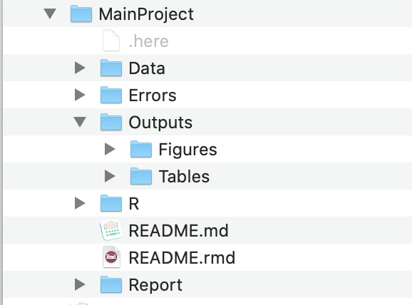
Here’s what my project folders tend to look like (figure below). And here is a template GitHub repo to show what the structure typically looks like.

It should go without saying that sharing your data (if possible) and code will help you and your collaborators catch errors before it’s too late, but also, sharing them with others/the public after a project is done will also help catch possible errors that you/your collaborators/reviewers didn’t catch, which may mislead other researchers and also result in a much more stressful situation for you.

And last but not least, it is also essential to give extensive details on which version of R you used and which packages you used and their versions. This is because many scripts that once worked on previous versions of the software may no longer give the same results or may not even work at all. In order for someone to reproduce your results, they’ll need to know the environment on which you ran your analyses on. You can provide these details easily simply by running the script sessionInfo(), which should be at the end of every R script you run.

4 Helpful Resources

Workflow for Statistical Analysis and Report Writing

How to Save Data File into .RData?

Basic Data Entry Using Excel

Sending Me Data in Excel

Happy Git and GitHub for the useR

5 Environment

The analyses were run on:

#> R version 4.5.0 (2025-04-11)
#> Platform: aarch64-apple-darwin20
#> Running under: macOS Sequoia 15.6.1
#> 
#> Matrix products: default
#> BLAS:   /Library/Frameworks/R.framework/Versions/4.5-arm64/Resources/lib/libRblas.0.dylib 
#> LAPACK: /Library/Frameworks/R.framework/Versions/4.5-arm64/Resources/lib/libRlapack.dylib;  LAPACK version 3.12.1
#> 
#> Random number generation:
#>  RNG:     Mersenne-Twister 
#>  Normal:  Inversion 
#>  Sample:  Rejection 
#>  
#> locale:
#> [1] en_US.UTF-8/en_US.UTF-8/en_US.UTF-8/C/en_US.UTF-8/en_US.UTF-8
#> 
#> time zone: America/New_York
#> tzcode source: internal
#> 
#> attached base packages:
#> [1] stats     graphics  grDevices utils     datasets  methods   base     
#> 
#> loaded via a namespace (and not attached):
#>  [1] htmlwidgets_1.6.4 compiler_4.5.0    fastmap_1.2.0     cli_3.6.5        
#>  [5] tools_4.5.0       htmltools_0.5.8.1 rstudioapi_0.17.1 yaml_2.3.10      
#>  [9] rmarkdown_2.29    knitr_1.50        jsonlite_2.0.0    xfun_0.53        
#> [13] digest_0.6.37     rlang_1.1.6       evaluate_1.0.5

6 References

--- layout: post title: 'Quality Control in Statistical Analyses' author: 'Zad Rafi' date: 2020-06-13 lastmod: "`r Sys.Date()`" description: "Experienced statisticians and data analysts are familiar with stories where a coding error has led to an entire conclusion changing, even leading to a retraction. It's the sort of stuff that keeps people up at night." archives: statistics slug: statistics-quality-control url: statistics/statistics-quality-control zotero: true categories: - statistics tags: - statistical reporting - statistical science - statistical workflow - data management image: https://res.cloudinary.com/less-likely/image/upload/v1613136545/Site/diagram.png og_image: https://res.cloudinary.com/less-likely/image/upload/v1613136545/Site/diagram.png keywords: - statistical reporting - statistics - accuracy - data science codefolding_show: "show" output: blogdown::html_page: toc: true --- ```{r setup, include = FALSE, message=FALSE} knitr::opts_chunk$set( collapse = TRUE, comment = "#>") ``` ------------------------------------------------------------------------ Experienced statisticians and data analysts are familiar with stories where a coding error has led to an entire conclusion changing, [or even a retraction](https://jamanetwork.com/journals/jama/fullarticle/2752474).\[\@aboumatarNoticeRetractionAboumatar2019\] It's the sort of stuff that keeps people up at night. Unfortunately, not many of us think about these sorts of scenarios until we realize it's very possible that it could happen to any of us. To me, it seems that many of these issues could be avoided by having a principled data management and statistical workflow, and making it as transparent, open, and reproducible as possible. I'd like to quickly go over a few things that I've found helpful over the years, and I'll first start with data management and data entry and then move onto analysis workflows. I largely consider this to be a living document, and I'm sure many people who will read this will have far better suggestions, so please leave them down below in the comments! Before I go on, I want to emphasize that backing up your data, scripts, and [using version control](https://happygitwithr.com/) is extremely important. There is no debate about this. It's necessary so that other collaborators/colleagues can inspect your work and catch potential mistakes or see overall progress, but more importantly, it will prevent you from losing your data in a disaster, and it'll help you catch your own mistakes, since you'll be the most familiar with the data and scripts. ------------------------------------------------------------------------ # Data Entry & Management ------------------------------------------------------------------------ A nice paper that I'd like to review is the one by [Broman & Woo, 2018](https://doi.org/10.1080/00031305.2017.1375989) on how to manage your data when working with spreadsheets.\[\@bromanDataOrganizationSpreadsheets2018\] The sad reality is that even though spreadsheets like Microsoft Excel or Google Sheets are available everywhere, and easy to use, there are many risks when working with spreadsheets, just ask any [statistician who works in genetics](https://genomebiology.biomedcentral.com/articles/10.1186/s13059-016-1044-7?fbclid=IwAR06eQ5LTg2LX5byJBWfC6rJdAbAGXKvy3PUOhzPsVjUGqb7KqB1V_x36M0) or any bioinformatician.\[\@ziemannGeneNameErrors2016\] One of the most fatal errors [occurred recently](https://theconversation.com/why-you-should-never-use-microsoft-excel-to-count-coronavirus-cases-147681) when a group of researchers lost thousands of documented COVID cases because they entered data for each case as a column instead of a row, and Excel has a limit on how many columns and rows it can handle (**1,048,576 rows** and **16,384 columns**, [according to Microsoft](https://support.microsoft.com/en-us/office/excel-specifications-and-limits-1672b34d-7043-467e-8e27-269d656771c3)), as a result, most of these cases were lost, resulting in an enormous waste of resources due to a careless and ignorant mistake, highlighting the dangers of recklessly inputting data and conducting statistical analyses. There is no doubt that reviewing principles of good data management and workflow are essential to any data analyst. I'd like to touch on some of the most important points of [Broman & Woo, 2018](https://doi.org/10.1080/00031305.2017.1375989) paper before moving onto some other "principles" I'd like to share: ------------------------------------------------------------------------ ## General Principle: Be Consistent With Everything ------------------------------------------------------------------------ <html> - When labeling missing values (`NA`, `N/A`, etc.): - Good: Choose one method (`NA`, `N/A`, etc.) and stick with it. - Bad: Leaving cells empty to indicate missingness. * * * - When labeling response variables: - Good: If you label a response variable consistently, for example, `fat-free-mass` in every instance to refer to the same variable. - Bad: If you label a response variable `fat-free-mass` in one script/sheet, and `ffm`/`fat_free_mass` in another. * * * - When formatting variable predictor names: - Good: `predictor_1_week12`, `predictor_2_week12`, `response_variable_week12`. This is consistent, with the order of the names, and dates/weeks, so it is easier to organize, inspect, and clean. Same thing applies to labeling response variables and pretty much all variables. - Bad: When you label one variable `week12_predictor_1`, the next `predictor_2_week12`, and the last, `12_week_response`. Just _no_. * * * - When formatting dates: - Good: Use one format, `YYYY-MM-DD`, consistently. - Bad: Everything else. * * * - When filling out cells: - Good: One cell = one thing. No more, no less. - Bad: One cell = multiple entries or no entries at all. * * * - When keeping track of the data: - Good: Create a comprehensive data dictionary so anyone can look at it and understand the spreadsheets/dataframes/variables. - Bad: Expecting yourself and others to figure it out based on the variable names that you thought were brilliant. * * * - When using Excel or Google Sheet's shiny features: - Good: Avoid using any of them, any formulas, highlighting, _italicizing_, bolding, etc. - Bad: If you're the type of person to create charts in Excel. * * * - Planning for disasters: - Good: Always, always, backup your files, save them in .txt files. Keep backups of those. And most importantly, [**use version control!**](https://happygitwithr.com/) - Bad: You don't really plan for disasters and go with the flow. </html> ------------------------------------------------------------------------ - Last but not least, when entering cases: - Good: Rows are for cases and observations, and columns are for variables and characteristics. Please do not switch these up! - Bad: Using them interchangeably. ------------------------------------------------------------------------ # Setting Up a Principled Statistical Workflow ------------------------------------------------------------------------ Here's what I've been doing for many years and what seems to work for me (none of these ideas are originally mine, and I actually picked them up over the years from others' advice, which will be linked below). ------------------------------------------------------------------------ ## Setting up the Project Folder ------------------------------------------------------------------------ When setting up a folder specific for a project (if you're not doing this, you absolutely need to), first, I will create a folder with the title of my project, and usually have an [`RStudio`](https://rstudio.com/) project set up in there. ------------------------------------------------------------------------ > Disclaimer: while much of this advice will be familiar and easy to > understand for those who use `R`, I think the general principles are > widely applicable, especially for those who use scripts in their > statistical software). ------------------------------------------------------------------------ This folder will contain many other folders (more on that below), so the structure will end up being a bit complex. ------------------------------------------------------------------------ ```{r Structure of Workflow, eval=FALSE, include=FALSE} diagram <- DiagrammeR::grViz("digraph { graph [layout = dot, rankdir = TB, compound = true, nodesep = .5, ranksep = .25] node [shape = circle, fixedsize = true, fontsize = 9.5, fontname = Helvetica, fontcolor = '#000000', width = .99, height = .99, style = filled, color = '#91A3B0', label = ''] edge [color = grey, arrowhead = normal, arrowtail = inv] rec1 [label = 'Main Project \nFolder'] rec2 [label = 'Data \nFolder', fillcolor = '#3f8f9b'] rec3 [label = 'R Scripts \nFolder', fillcolor = '#7aa864'] rec4 [label = 'Errors \nFolder', fillcolor = '#d46c5b'] rec5 [label = 'Outputs \nFolder', fillcolor = '#E69F00'] rec6 [label = 'README.md \nFile', fillcolor = pink] rec7 [label = '.here \nFile', fillcolor = white] rec8 [label = 'Reports \nFolder', fillcolor = '#91A3B0'] rec9 [label = 'Stored Models \nFolder', fillcolor = '#3f8f9b'] rec10 [label = 'source.R', fillcolor = '#7aa864'] rec11 [label = '02-cleaning.txt', fillcolor = '#d46c5b'] rec12 [label = 'Figures \nFolder', fillcolor = '#E69F00'] rec13 [label = 'HTML Files \nFolder', fillcolor = '#91A3B0'] rec14 [label = 'Spreadsheets \nFolder', fillcolor = '#3f8f9b'] rec15 [label = '01-functions.R', fillcolor = '#7aa864'] rec16 [label = '03-inspection.txt', fillcolor = '#d46c5b'] rec17 [label = 'Tables \nFolder', fillcolor = '#E69F00'] rec18 [label = 'Text Files \nFolder', fillcolor = '#3f8f9b'] rec19 [label = '02-cleaning.R', fillcolor = '#7aa864'] rec20 [label = '04-analysis.txt', fillcolor = '#d46c5b'] rec21 [label = 'Manuscripts \nFolder', fillcolor = '#91A3B0'] rec22 [label = '03-inspection.R', fillcolor = '#7aa864'] rec23 [label = '05-sensitivity.txt', fillcolor = '#d46c5b'] rec24 [label = 'LaTeX Files \nFolder', fillcolor = '#91A3B0'] rec25 [label = '04-analysis.R', fillcolor = '#7aa864'] rec26 [label = '06-tables.txt', fillcolor = '#d46c5b'] rec27 [label = '05-sensitivity.R', fillcolor = '#7aa864'] rec28 [label = '06-tables.R', fillcolor = '#7aa864'] rec29 [label = '.git Files ', fillcolor = white] # edge definitions with the node IDs {rec7 rec6 rec29} -> rec1 -> {rec2 rec3 rec4 rec5 rec8} {rec3 -> rec10} {rec10-> rec15-> rec19-> rec22} {rec10 -> rec25-> rec27-> rec28} rec5 -> {rec12 rec17} rec8 -> {rec13 rec21} rec21-> rec24 rec2 -> {rec9 rec14 rec18} rec4 -> rec11-> rec16 rec4 -> rec20-> rec23-> rec26 } ", height = 700, width = 700) library(vtree) diagram1 <- grVizToImageFile(diagram, width = NULL, height = NULL, format ="pdf", folder = ".", filename = "diagram.pdf") diagram2 <- grVizToImageFile(diagram, width = NULL, height = NULL, format ="png", folder = ".", filename = "diagram.png") pdftools::pdf_convert("/Users/zad/Desktop/GitHub/LessLikely/content/post/statistics/diagram.pdf", "png", 1, "/Users/zad/Desktop/GitHub/LessLikely/content/post/statistics/diagram.png") ``` ```{r eval=FALSE, include = FALSE, fig.height=5, fig.width=5} library(knitr) library(magrittr) URL <- "~/Desktop/GitHub/LessLikely/content/post/statistics/diagram.pdf" URL2 <- "~/Desktop/GitHub/LessLikely/content/post/statistics/diagram.png" include_graphics(URL, auto_pdf = T, error = T) %>% render_markdown(strict = FALSE) ``` <img data-enlargeable style="cursor: zoom-in" src="https://res.cloudinary.com/less-likely/image/upload/v1613136545/Site/diagram.png" alt="workflow"/> ------------------------------------------------------------------------ > It may be a bit difficult to read the words within the circles, but > clicking on the diagram should enlargen it and allow you to zoom in, > giving you a sense of how I organize all these scripts and files. ------------------------------------------------------------------------ If this ends up confusing you, you can just scroll all the way down to see an image of what the folder structure looks like. Instead of constantly changing the working directory to each subfolder when I need to do something inside that subfolder for a particular project or analysis, I set the project folder as the working directory only once, and then run the following: ------------------------------------------------------------------------ ```{r Setting Project Folder, eval=FALSE, include=TRUE} # Very seriously consider installing the `here` package # https://cran.r-project.org/package=here library("here") # This and the scripts below take # the directory used and set it as the top set_here() here() ``` ------------------------------------------------------------------------ This not only sets the working directory, but gives you far more control over how you can save your files from any place within the hierarchical folder structure. It will create a file called `.here` inside the `Main Project` folder, which will indicate that this is the top level of the hierarchy. Then, I will usually have created a `README.Rmd` file in the `Main Project` folder with updates on what I've done and what I still need to work on, so I will remember and so my collaborators can see it too (when it has been pushed to GitHub or other [version control](https://happygitwithr.com/) repos). Next, I'll set up a `Data` folder inside the `Main Project` folder. This is where all my data/spreadsheets/.txt files and data dictionaries will go. The original data files will stay inside this folder, while I create two other subsubfolders inside this `Data` folder called `Transformed` and `Models`. In `Transformed`, I will typically save `.rds` files that were a result of cleaning and transforming the data, including imputing missing data. I will touch more on exactly how I do that later below. A `Models` subfolder will obviously store fitted models and any validation/sensitivity analyses of those models.\[\@morrisChoosingSensitivityAnalyses2014\] Now, back to the `Main Project` folder, I'll set up another folder within it called `R`. This will be where all of my `.R` scripts/files live. I will number them sequentially along with a title for a specific purpose, like so ------------------------------------------------------------------------ - `main.R` - `01-functions.R` - `02-cleaning.R` - `03-inspection.R` - `04-analysis.R` - `04.5-validation.R` - `05-sensitivity.R` - `06-tables.R` ------------------------------------------------------------------------ ## Setting up the Functions Script ------------------------------------------------------------------------ All potential `R` packages and custom functions that I need will belong in `01-functions.R`. This `.R` file will only serve this purpose and nothing else. As you've guessed by now, the other `.R` files will be doing the same, they have very specific purposes and are organized to reflect this. An example of the first script can be found below. ------------------------------------------------------------------------ ```{r Beginning Functions Script, eval=FALSE, include=TRUE} # Necessary Packages ------------------------------------ req_packs <- c("rms", "concurve", "mice", "tidyverse", "parallel", "bayesplot", "projpred", "Hmisc", "loo", "rstan", "here", "tryCatchLog", "futile.logger", "patchwork", "corrplot", "beepr", "summarytools", "broom", "wakefield", "boot", "mfp", "knitr", "flextable", "MASS", "lme4", "brms", "miceMNAR") # Load all packages at once lapply(req_packs, library, character.only = TRUE) # Loggings messages options(keep.source = TRUE) options("tryCatchLog.write.error.dump.file" = TRUE) # Set seed for random number generator RNGkind(kind = "L'Ecuyer-CMRG") set.seed(1031) # My birthday # RStan Settings ------------------------------------- theme_set(theme_bw()) color_scheme_set("red") rstan_options(auto_write = TRUE) options(mc.cores = 4) has_build_tools(debug = TRUE) # Stan Settings --------------------------------------- dotR <- file.path(Sys.getenv("HOME"), ".R") if (!file.exists(dotR)) dir.create(dotR) M <- file.path(dotR, "Makevars") if (!file.exists(M)) file.create(M) cat("\nCXX14FLAGS=-O3 -march=native -mtune=native -fPIC", "CXX14=g++", file = M, sep = "\n", append = TRUE) ``` ------------------------------------------------------------------------ The script above loads all the necessary `R` packages each time it is called, along with the specified functions, so most of the other `.R` files will depend upon this one. However, I will not be running each of these `.R` files/scripts individually, line by line, or by selecting all the lines in an `.R` file and running the script. Instead, after I've created all these files (figuring out what I need to do carefully and writing it down and annotating it), every single `.R` file except for `main.R` will have the following script, which I will explain later below (or some iteration of this script to match the name of the file) at the beginning: ------------------------------------------------------------------------ ## Setting up the Error Catching Script ------------------------------------------------------------------------ ```{r Beginning Error Script, eval=FALSE, include=TRUE} library("here") set_here() source(here("R", "01-functions.R")) library(futile.logger) library(tryCatchLog) # Keeps source code file name and line number tracking options(keep.source = TRUE) options("tryCatchLog.write.error.dump.file" = TRUE) # Logs messages into a file flog.appender(appender.file("my_app.log")) flog.threshold(INFO) # Function that catches any messages tryCatchLog(source("script.R")) ``` ------------------------------------------------------------------------ You'll notice several things. First, I'm once again calling the [`here`](https://cran.r-project.org/package=here) package and telling it that I'm working within this folder (`R`), and then I'm calling the `01-functions.R` file by using the `source()` function, but also notice how the `source()` function is followed by a `here()` function/argument. This `here()` function allows you to fully control files in a specific folder from anywhere else, without having to actually be in that folder. So, suppose I was in the `Main Project` -\> `Data` -\> `Models` folder and I was saving my work there (in the `Models` folder), which is pretty far from the `R` folder, I can still, using functions like `source()`, `save()`, etc., call or manipulate files from a totally different folder by specifying the hierarchy using `here()`. This can also be done in other ways, but those are far more cumbersome, and not flexible. This is how I always call the necessary packages and functions I need from every `.R` script, simply by using the `source()` function and using `here()` to direct it to the `01-functions.R` file in the `R` folder. Now let's look at the next few lines. ------------------------------------------------------------------------ ```{r Error Script, eval=FALSE, include=TRUE} flog.appender(appender.file("script.log")) flog.threshold(INFO) tryCatchLog(source("script.R")) ``` ------------------------------------------------------------------------ This script is designed to catch any warnings that occur inside the `.R` script and save them to a .log file in another subfolder within the `R` folder called `Errors`. So here's an example of a full script for a mix of data generation and inspection, so that you can see it in action. ------------------------------------------------------------------------ ## Example of Data Loading & Inspection ------------------------------------------------------------------------ ```{r Example 1, eval=FALSE, include=TRUE} library("here") set_here() source(here("R", "01-functions.R")) # Loads all R functions # First we need some data RNGkind(kind = "L'Ecuyer-CMRG") set.seed(1031) # My birthday # Suppose you wanted to simulate a clinical trial library("simstudy") # Simulating a Clinical Trial -------------------------- def <- defData(varname = "male", dist = "binary", formula = .5 , id="cid") def <- defData(def, varname = "over65", dist = "binary", formula = "-1.7 + .8 * male", link = "logit") def <- defData(def,varname = "baseDBP", dist = "normal", formula = 70, variance = 40) def <- defData(def, varname = "age", dist = "normal", formula = 10, variance = 2) def <- defData(def, varname = "visits", dist = "poisson", formula = "1.5 - 0.2 * age + 0.5 * male", link = "log") def <- defData(def, varname = "weight", dist = "normal", formula = 60, variance = 10) dtstudy <- genData(500, def) study <- trtAssign(dtstudy, nTrt = 2, balanced = FALSE, grpName = "rxGrp") study <- as.data.frame(study) study$iq <- iq <- wakefield::iq(500) study$height <- height <- wakefield::height(500) study$income <- income <- wakefield::income(500, digits = 2, name = "Income") study$SAT_score <- wakefield::sat(500, mean = 1500, sd = 100, min = 0, max = 2400, digits = 0, name = "SAT") study$visits <- as.numeric(study$visits) # Add noisy predictors study[, 11:20] <- lapply(1:10, FUN = function(i) (rnorm(n = 500, mean = 1, sd = 2))) varname <- sprintf("x%d", (11:20)) colnames(study)[11:20] <- varname study1 <- trtAssign(dtstudy, n = 2, balanced = TRUE, strata = c("male", "over65"), grpName = "rxGrp") study1 # Inspecting Data ------------------------------------- summarytools::view(dfSummary(study)) study$over65 <- as.factor(study$over65) study$male <- as.factor(study$male) study$rxGrp <- as.factor(study$rxGrp) study_formula <- as.formula(baseDBP ~ .) plot(spearman2(study_formula, study)) abline(v = 0) x_1 <- model.matrix(~ ., data = study)[, -1] # Initial Data Analysis ------------------------------ (cormatrix <- (cor(x_1))) col <- colorRampPalette(c("#BB4444", "#EE9988", "#FFFFFF", "#77AADD", "#4477AA")) corrplot(cormatrix, method = "color", col = col(200), tl.col = "black", tl.cex = 0.40, addCoef.col = "black", number.cex = .35) clus1 <- varclus(x_1, similarity = "h") clus2 <- varclus(x_1, similarity = "s") clus3 <- varclus(x_1, similarity = "p") plot(clus1, ylab = "Hoeffing's D statistic", lwd = 2.5, lty = 1, cex = 0.75) title("Hierarchical Cluster Analysis") plot(clus2, lwd = 2.5, lty = 1, cex = 0.75) plot(clus3, lwd = 2.5, lty = 1, cex = 0.75) Pre <- names(study) (fmla <- as.formula(paste("~", paste(Pre, collapse = "+")))) # Redundancy analysis redun <- redun(fmla, data = study, r2 = 0.90, type = "ordinary", allcat = FALSE, tlinear = FALSE, iterms = FALSE, pr = TRUE) ``` ------------------------------------------------------------------------ The above script simulated some fake data for a hypothetical clinical trial (usually we use this first script to load data from a .csv or .txt file) and then we used several functions to inspect the dataframe for the structure and distributions of the variables and missing data, etc. We also attempted to properly code the variables. Now, in order to capture any possible errors, we will have to run this entire script from another `R` script instead of running it line by line or selecting all the code and running it. We will do this from a Main source script, which will allow us to use the `tryCatchLog()` function. ------------------------------------------------------------------------ ## Example of the Main Source Script ------------------------------------------------------------------------ ```{r Main Source Script, eval=FALSE, include=TRUE} library("here") library("tryCatchLog") library("futile.logger") set_here() # Load and set here here() # Call here options(keep.source = TRUE) options("tryCatchLog.write.error.dump.file" = TRUE) # Script loads all necessary functions flog.appender(appender.file( here("Errors", "01-functions.log"))) tryCatchLog(source(here("R", "01-functions.R"))) # Line script to clean the data flog.appender(appender.file( here("Errors", "02-cleaning.log"))) tryCatchLog(source(here("R", "02-cleaning.R"))) # Line script below to inspect the data flog.appender(appender.file( here("Errors", "03-inspection.log"))) tryCatchLog(source(here("R", "03-inspection.R"))) # Load saved objects from cleanings flog.appender(appender.file( here("Errors", "03.5-load_data.log"))) tryCatchLog(source(here("R", "03.5-load_data.R"))) # Main analysis script flog.appender(appender.file( here("Errors", "04-analysis.log"))) tryCatchLog(source(here("R", "04-analysis.R"))) # Below is the validation of main analysis results flog.appender(appender.file( here("Errors", "04.5-validation.log"))) tryCatchLog(source(here("R", "04.5-validation.R"))) # Test the sensitivity of the results by # varying assumptions/multiple parameters flog.appender(appender.file( here("Errors", "05-sensitivity.log"))) tryCatchLog(source(here("R", "05-sensitivity.R"))) # Generate tables and figures of all your results flog.appender(appender.file( here("Errors", "06-tables.log"))) tryCatchLog(source(here("R", "06-tables.R"))) # Export these into actual files that can be # inserted into papers, reports, etc. flog.appender(appender.file( here("Errors", "07-export.log"))) tryCatchLog(source(here("R", "07-export.R"))) ``` ------------------------------------------------------------------------ If anything went wrong during the simulations and their inspections in the first script from above, it would have been captured by the error-catching scripts that we have set up, which would be placed within a .log file in the `Errors` folder, which is inside the `R` folder. ------------------------------------------------------------------------ ## Setting the Seed ------------------------------------------------------------------------ > Also, note that we have set the seed using a specific random number > generator algorithm. This is not that important, however, it is > important to correctly set the seed for reproducing any random numbers > generated. This requires even more careful thought when running a > simulation study, in which the states of the simulation need to be > saved for a particular repetition, and so that streams do not > overlap.\[\@morrisUsingSimulationStudies2019\] ------------------------------------------------------------------------ I will admit that the error script is not *perfect* at capturing warnings, but for most things, if something wrong occurs when a script is run, the function `tryCatchLog()` and its .log file usually catches the warning, so I would know that something went wrong and what specifically. However, some may be skeptical of this approach and ask why I need to catch these errors and save them if I ran the scripts? Why not just scroll up and look at the console to see the errors or warnings? Many reasons: ------------------------------------------------------------------------ - Suppose the analyses take a very long time, and are computationally intensive, and `R`/[`RStudio`](https://rstudio.com/) crashes, you may not be able to figure out what went wrong. - Suppose the analysis completed but because there was so much occurring in the console (for example, sampling from a posterior) that you missed the warnings/errors and got results that you don't know have issues. ------------------------------------------------------------------------ Thus, having this system set up to catch errors in every script also helps us automate the entire workflow once we've carefully set it up. After each `.R` script has one of these message-catching scripts, we can run our entire analysis from start to finish from `main.R` with one command. This not only makes your workspace organized, but also makes it easier for others to reproduce your work if you share your files and folders via a repository. ------------------------------------------------------------------------ So, now the `Error` folder will contain .txt files with any warning messages or errors. Typically, when I'm setting up a new project, I will also add a few other folders such as an `Outputs` folder, where I will save tables and graphs, and a `Report` folder, where I might be working on a manuscript. Now that I've mentioned my hierarchy and how I catch errors, I can mention some other things that I believe are absolutely heinous practices. Many people often will run an entire analysis and have several objects/vectors stored in their Global Environment in `R` and `RStudio`. Suppose they're taking a break, finished with the analysis, turning off the computer, or stepping away for whatever reason, what they'll typically do is click the save button on the top right pane and "Save the workspace image". Indeed, if they don't do that themselves, the IDE `RStudio` will explicitly ask them if they wish to save their workspace image. This is a horrific practice and you should never do this because it can lead to several problems such as: - having several saved objects and packages conflict with one another once they're all loaded together at once - having giant workspace images, that will probably cause `R`, and especially `RStudio` to constantly crash - not allowing you to load very specific objects that you need at a time while leaving everything else I would say that it is a good idea to never save the workspace image, ever. It is also quite easy to turn off. Simply go the `RStudio` menu and click *Preferences*, and in the *General* section, you will see the following options: ------------------------------------------------------------------------ <img data-enlargeable width="500" style="cursor: zoom-in" src ="https://res.cloudinary.com/less-likely/image/upload/v1604649526/Site/RStudio_Default_Save_Options.png"> ------------------------------------------------------------------------ It is essential to uncheck everything under *R Sessions*, *Workspace*, and *History*, so that you do not set your self up for a future disaster. Instead of using these convenient but highly problematic options, always use the `saveRDS()` base `R` function, where the first argument is the object in your environment that you want to save, and the second argument is the path where you want to save it, which of course should be using the `here()` function. Now suppose I decided to use multiple imputation because I had a dataset with many missing values, and suppose I had a grasp of the missing data mechanism, and so I used something like the not-at-random fully conditional specification approach (**NARFCS**)\[\@tompsettUseNotatrandomFully2018\] to attempt to handle data that I believe to be missing not at random (**MNAR**), and I wanted to save the imputed dataset, and only load the imputed dataset next time. This is how I would do it (in the vaguest way possible). First, I'll start with the dataset that we generated above and generate missing values via different missing data mechanisms using the `ampute()` function from the `mice` package.\[\@buurenMiceMultivariateImputation2011\] ------------------------------------------------------------------------ > **Important**: This is all assuming that one has carefully constructed > an imputation model, and that multiple imputation is the most > appropriate solution. As many others have pointed out, simply running > a script like `mice(data)` in `R` without careful thought to the > imputation model, is a very, very bad idea. Missing data is an > extremely complex topic and I recommend everyone carefully read the > works\[\@buurenFlexibleImputationMissing2018\] of missing data > researchers such as: - [Stef van Buuren](https://stefvanbuuren.name/fimd/) > - [Tim Morris](https://twitter.com/tmorris_mrc) > - [Ian White](https://www.ctu.mrc.ac.uk/about-us/senior-staff/ian-white/) > - [Donald Rubin](https://scholar.google.com/citations?user=5q4fhUoAAAAJ&hl=en) > - [Jonathan Bartlett](https://thestatsgeek.com/) > - [Paul Gustafson](https://www.paulgstf.com/) > ------------------------------------------------------------------------ ## Example of a Multiple Imputation Script ------------------------------------------------------------------------ ```{r Example of Imputing Data, eval=FALSE, include=TRUE} source(here("R", "01-functions.R")) library("beepr") # Package that uses multiple imputation # by chained equations library("mice") # Generate Missing Data -------------------------------- study_mnar <- ampute(data = study[, 5:10], prop = 0.65, mech = "MNAR") mnar_patterns <- study_mnar$patterns mnar_weight <- study_mnar$weight study_mnar_rerun <- ampute(data = study[, 5:10], prop = 0.5, mech = "MNAR", patterns = mnar_patterns, weights = mnar_weight) study_mar <- ampute(data = study[, 2:4], prop = 0.5, mech = "MAR") mar_patterns <- study_mar$patterns mar_weight <- study_mar$weight study_mar_rerun <- ampute(data = study[, 2:4], prop = 0.5, mech = "MAR", patterns = mar_patterns, weights = mar_weight) study_mar_rerun[[11]]$over65 %>% as.factor() study_mar_rerun[[11]]$male %>% as.factor() study_mar_rerun[[11]]$rxGrp %>% as.factor() df <- study_mnar_rerun$amp df2 <- study_mar_rerun$amp # Inspect Data str(df) # Inspect data frame summary(df) # High level summary of dataframe sum(is.na(df)) # Look at missing values etc. colSums(is.na(df)) summarytools::view(dfSummary(df)) str(df2) # Inspect data frame summary(df2) # High level summary of dataframe sum(is.na(df2)) # Look at missing values etc. colSums(is.na(df2)) summarytools::view(dfSummary(df2)) # Prepare Data for Imputation ------------------------- temp <- df temp2 <- df2 missing_plot(temp) missing_plot(temp2) # Set-up predictor matrix predMatrix <- make.predictorMatrix(temp) predMatrix2 <- make.predictorMatrix(temp2) # Set-up predictor matrix for unidentifiable part: predSens <- matrix(rep(0, 6), ncol = 6, nrow = 6) colnames(predSens) <- paste(":", names(temp), sep = "") rownames(predSens) <- names(temp) # Set-up list with sensitivity parameter values pSens <- rep(list(list("")), ncol(temp)) names(pSens) <- names(temp) pSens[["rxGrp"]] <- list(-.4) pSens[["baseDBP"]] <- list(-.4) pSens[["male"]] <- list(-.4) pSens[["over65"]] <- list(-.2) # MICE RI Imputation ---------------------------------- z1 <- parlmice(data = temp, method = "ri", predictorMatrix = predMatrix, m = 8, maxit = 1, cluster.seed = 1031, n.core = 4, n.imp.core = 2, cl.type = "FORK", ridge = 1e-04, remove.collinear = TRUE, remove.constant = FALSE, allow.na = TRUE) z2 <- parlmice(data = temp2, method = "pmm", predictorMatrix = predMatrix2, m = 8, maxit = 1, cluster.seed = 1031, n.core = 4, ridge = 1e-04, remove.collinear = TRUE, n.imp.core = 2, cl.type = "FORK") zfinal <- cbind(z1, z2) # Heckman Imputation ---------------------------------- study$baseDBP <- temp$baseDBP JointModelEq<-generate_JointModelEq(data=temp, varMNAR="baseDBP") JointModelEq[,"baseDBP_var_sel"] <- c(0,1,1,1,1,1) JointModelEq[,"baseDBP_var_out"] <- c(0,1,1,1,1,1) arg <- MNARargument(data = temp, varMNAR = "baseDBP", JointModelEq = JointModelEq) arg$method["age"] <- "ri" arg$method["visits"] <- "ri" arg$method["weight"] <- "ri" arg$method["iq"] <- "ri" arg$method["height"] <- "ri" imp1 <- parlmice(data = arg$data_mod, method = arg$method, predictorMatrix = arg$predictorMatrix, JointModelEq = arg$JointModelEq, control = arg$control, maxit = 1, m = 8, cluster.seed = 1031, n.core = 4, n.imp.core = 2, cl.type = "FORK") analysis1 <- with(zfinal, glm(baseDBP ~ age + visits + weight + iq + height + rxGrp + male + over65)) result1 <- pool(analysis1) summary(result1) z2 <- parlmice(data = temp2, method = "pmm", predictorMatrix = predMatrix2, m = 8, maxit = 1, cluster.seed = 1031, n.core = 4, n.imp.core = 2, cl.type = "FORK") heckman <- cbind(imp1, z2) beep(3) # I will touch on this function below. saveRDS(zfinal, here("Main Project", "Data", "zfinal.rds")) ``` ------------------------------------------------------------------------ Here is the workflow truly showing its advantages, `saveRDS()` is saving a very specific object (`zfinal`, the imputed dataset) into the `Data` folder by using the hierarchical structure of the folder which can easily be navigated using `here()`. Notice how to save something and use `here()` to specify the location, the first argument is `Main Project`, followed by `Data`, and then comes the object name (`zfinal.rds`). Now I have saved my imputed dataset as an object called `zfinal.rds` and it is saved in the `Data` folder even though I am hypothetically working from the `R` folder. Also notice that I use the `beep()` function from the [beepr](https://cran.r-project.org/package=beepr) `R` package, which can be quite handy in letting you know if a particular script or analysis is done. Next time, if I cleared my entire global environment and wanted to only load the imputed dataset, I would simply have to just click on the `zfinal.rds` file in the `Data` folder and it would load into the environment or I could use the following command, ------------------------------------------------------------------------ ## Saving and Reading Data Carefully ------------------------------------------------------------------------ ```{r Reading Saved Data, eval=FALSE, include=TRUE} # The function readRDS() and saveRDS() # are possibly the most important base R functions zfinal <- readRDS("zfinal.rds", here("Main Project", "Data", "zfinal.rds")) ``` ------------------------------------------------------------------------ This gives us full control over the environment, and it's also why I encourage people to turn off the automatic prompt to save the workspace that [`RStudio`](https://rstudio.com/) gives you by default (I am certain even Hadley Wickham has said the same on multiple occasions). So if I now wanted to include the imputed dataset into one of my `.R` scripts that I am trying to automate with one command, whether for reproducibility, or speed, etc., I could do it with absolute control. This is also how I save my models and how I validate them, which is especially handy because running those can also take an excruciatingly long time. Here's an example of a script that would be in the `04-analysis.R` script, I'm leaving out the warning-catching script now to avoid making this too long. I don't need to load the [`brms`](https://cran.r-project.org/package=brms) package because I'm already calling it from the first `.R` script, `01-functions.R` (but I'm just showing it for now to avoid confusion), and then I am saving it in the `Models` folder which is found in the `Data` folder. And again, the `beep()` function would let me know when the script is over, and scripts like this can often take very long, due to the computational intensity. The script below is an analysis script whose results we plan on saving once completed. Due to the arguments I have set (iterations, warmups, chains, and using an imputed dataset), it can often take a long time before it is finished, and if I did happen to do other tasks while I was waiting on that, the output would automatically save to the `Models` folder via `saveRDS()`, and I would also receive a notification via the `beep()` function, preventing me from wasting any time. ------------------------------------------------------------------------ ## Example Modeling Script ------------------------------------------------------------------------ ```{r Analysis Script, eval=FALSE, include=TRUE} # Calling all packages, please report for duty source(here("R", "01-functions.R")) library("brms") # This is a script I used previously # where I used Bayes for regularization # Although these are all generic options # Prior Information -------------------------------- sample_z <- complete(zfinal, 1) n_1 <- nrow(sample_z) # of observations k_1 <- (ncol(sample_z) - 1) # of predictors p0_1 <- 2 # Prior for the number of relevant variables tau0_1 <- p0_1 / (k_1 - p0_1) * 1 / sqrt(n_1) # tau scale # Regularized horseshoe prior hs_prior <- set_prior("horseshoe(scale_global = tau0_1, scale_slab = 1)", class = "b") library("future") plan(multiprocess) # Regularized Bayesian quantile # regression using regularized horseshoe prior brms::brm_multiple( bf(baseDBP ~ age + visits + weight + iq + height + rxGrp + male + over65, quantile = 0.50), data = zfinal, prior = hs_prior, family = asym_laplace(), sample_prior = TRUE, seed = 1031, future = F, iter = 1000, warmup = 500, chains = 4, cores = 4, thin = 1, combine = TRUE, control = list(max_treedepth = 10, adapt_delta = 0.80)) -> pen_model_1 # Principled way of saving results saveRDS(pen_model_1, here("Main Project", "Data", "Models", "pen_model_1.rds")) beep(3) ``` ------------------------------------------------------------------------ So I've saved the full contents of the fitted model (`pen_model_1`), which are usually several gigabytes large in size, within the `Models` folder. Once again, notice how the `here()` function allows you to work from a subfolder like `R`, which is inside the `Main Project` folder, and allows you to specify the hierarchy, and where you are within it, and save to whichever folder you wish, in this case `Models`, which is inside of `Data`. Now, I will typically conduct model checks and make sure it is performing well, and not misspecified, ------------------------------------------------------------------------ ```{r Checking, eval=FALSE, include=TRUE} source(here("R", "01-functions.R")) # Inspect RHat values --------------------------- rhats_1 <- pen_model_1$rhats rhats_1_df <- (rhats_1 <= 1.1) ((as.numeric(table(rhats_1_df)) / (nrow(rhats_1_df) * ncol(rhats_1_df)) * 100)) rhats_1_vec <- as.numeric(unlist(c( rhats_1[, 1:ncol(rhats_1)]))) pdf(here("Outputs", "Figures", "Diagnostics", "OUTCOME_COMP_rhat.pdf")) mcmc_rhat_hist(rhats_1_vec) + ggtitle("Model 1 Chain Convergence") dev.off() # Inspect Effective Sample Size ---------------------- mcmc_neff_hist(rhats_1_vec) + ggtitle("Effective Sample Size") # Inspect Divergences --------------------------- pdf(here("Outputs", "Figures", "Diagnostics", "OUTCOME_1.pdf")) mcmc_nuts_divergence(nuts_params(pen_model_1), log_posterior(pen_model_1)) dev.off() # Examine Residual Plots ---------------------------- df_resid_stan_1 <- data.frame(fitted(pen_model_1)[, 1], residuals(pen_model_1)[, 1]) pdf(here("Outputs", "Figures", "Diagnostics", "OUTCOME_1.pdf")) ggplot(df_resid_stan_1, aes(sample = residuals(pen_model_1)[, 1])) + geom_qq() + geom_qq_line() + ggtitle("Model 1 Residuals") dev.off() (sum1 <- (posterior_summary(pen_model_1))[2:8, ]) mcmc_intervals(pen_model_1, point_est = "median", prob = 0.95, prob_outer = 0, pars = parnames(pen_model_1)) + ggplot2::scale_y_discrete() + theme(axis.text=element_text(size=13), axis.title=element_text(size=13), plot.title = element_text(size=15, face = "bold")) + annotate("rect", xmin = -0.05, xmax = 0.05, ymin = 0, ymax = 7, fill = "darkred", alpha = 0.075) + annotate("segment", x = -0.05, xend = -0.05, y = 0, yend = 7, colour = "#990000", alpha = 0.4, size = .75, linetype = 3) + annotate("segment", x = 0.05, xend = 0.05, y = 0, yend = 7, colour = "#990000", alpha = 0.4, size = .75, linetype = 3) + ggtitle("Change in Outcome 1") dev.off() pdf(here("Outputs", "Figures", "OUTCOME_1.pdf")) mcmc_hist(pen_model_1) # Posterior Predictive Checks pdf(here("Outputs", "Figures", "Diagnostics", "OUTCOME_1check.pdf")) pp_check(pen_model_1, nsamples = 250) + ggtitle("Posterior Predictive Check: Model 1") dev.off() # Shows dens_overlay plot by default bayes_rsq1 <- bayes_R2(pen_model_1) bayes_rsq1 <- print(median(bayes_rsq1)) write.csv(sum1, here("Outputs", "Tables", "OUTCOME_1.csv")) ``` ------------------------------------------------------------------------ Once I have fit my model and done some initial checks, I usually conduct some more thorough checks using k-fold cross-validation or nested cross-validation, or bootstrap optimism. A script of this can be found below. ------------------------------------------------------------------------ ```{r, eval=FALSE, include=TRUE} source(here("R", "01-functions.R")) # 10-Fold Cross-Validations ------------------------- kfold_1 <- kfold(pen_model_1, K = 10, save_fits = TRUE, cores = 4) saveRDS(kfold_1, here("Data", "Models", "Validation", "kfold_1.rds")) kfp_1 <- kfold_predict(kfold_1) saveRDS(kfp_1, here("Data", "Models", "Validation", "kfp_1.rds")) kfold_rmse(y = kfp_1$y, yrep = kfp_1$yrep, type = "rmse", reps = 5000, cores = 4)[[2]][["t"]]) -> kfold_rmse_1 kfold_rmse_1 <- median(kfold_rmse_1) saveRDS(kfold_rmse_1, here("Data", "Models", "Validation", "kfold_rmse_1.rds")) ``` ------------------------------------------------------------------------ Once I've written all my analysis and validation scripts, I'll typically create a subfolder in the `Outputs` folder called `Figures` and `Tables` and save them appropriately with the help `here()`. ------------------------------------------------------------------------ ## Example Table Script ------------------------------------------------------------------------ ```{r Table Script, eval=FALSE, include=TRUE} source(here("R", "01-functions.R")) # Read in Validation Objects ------------------------ kfold_1 <- readRDS("kfold_1.rds", here("Main Project", "Data", "Models", "Validation", "kfold_1.rds")) kfold_2 <- readRDS("kfold_1.rds", here("Main Project", "Data", "Models", "Validation", "kfold_2.rds")) kfp_1 <- readRDS("kfp_1.rds", here("Main Project", "Data", "Models", "Validation", "kfp_1.rds")) kfp_2 <- readRDS("kfp_1.rds", here("Main Project", "Data", "Models","Validation", "kfp_2.rds")) # Extract Estimates from Objects --------------------- KFOLDIC_1 <- c(kfold_1[["estimates"]][3], kfold_2[["estimates"]][3]) KFOLDIC_SE_1 <- c(kfold_1[["estimates"]][3, 2], kfold_2[["estimates"]][3, 2]) BAYES_R2 <- c(bayes_rsq1, bayes_rsq2), 2) KFOLD_ELPD_1 <- c(kfold_1[["estimates"]][1], kfold_2[["estimates"]][1]) KFOLD_ELPD_SE_1 <- c(kfold_1[["estimates"]][1, 2], kfold_2[["estimates"]][1, 2]) Outcome <- c("OUTCOME_1", "OUTCOME_2") # Construct Data Frames ------------------------------ table4 <- data.frame(Outcome, BAYES_R2, KFOLD_ELPD_1, KFOLD_ELPD_SE_1, KFOLDIC_1, KFOLDIC_SE_1) colnames(table4) <- c("Outcome", "Bayes R^2", "10-fold CV ELPD", "10-fold CV ELPD SE", "10-fold CV IC", "10-fold CV IC SE") # Export as Tables ---------------------------------- write.csv(table4, here("Main Project","Outputs", "Tables", "Table4.csv")) table5 <- data.frame(Outcome, KFOLD_ELPD_1, KFOLD_ELPD_SE_1, KFOLDIC_1, KFOLDIC_SE_1) colnames(table5) <- c("Outcome", "10-fold CV ELPD", "10-fold CV ELPD SE", "10-fold CV IC", "10-fold CV IC SE") write.csv(table5, here("Main Project","Outputs", "Tables", "Table5.csv")) # Save Tables From Sensitivity Analyses -------------- write.csv(sens_table_OUTCOME_1, here("Main Project","Outputs", "Tables", "Table7_OUTCOME_1.csv")) write.csv(sens_table_OUTCOME_2, here("Main Project","Outputs", "Tables", "Table7_OUTCOME_2.csv")) ``` ------------------------------------------------------------------------ Then, I'll go back to the `README.Rmd` file, make notes of the hierarchy of the entire folder and subfolders, and what's been completed, and what still needs to be done. Now, suppose I deleted all of my saved models, imputed data, graphs, and tables, (which would be a devastating blow!) and only had the original dataset and organized scripts. Anyone could go into my project and simply highlight the entire `main.R` file and run it, and they would get all the same outputs and models, assuming a seed was set in advance, which is essential. Although, it might take them a long time to get the same outputs (if computationally intensive)... they would likely be able to get all the exact same results. ------------------------------------------------------------------------ # Possible Drawbacks of this Approach ------------------------------------------------------------------------ Every proposal tends to have drawbacks or limitations, and those who do not explicitly tell you about them are misleading you. In the approach I have outlined above, one major drawback is that it takes a somewhat long time to set up and therefore could deter many statisticians and data analysts. The other drawback is that by loading all your functions and libraries in the first `01_functions.R` script, there is potential for conflict between functions, therefore you'll have to be mindful of what packages you need and when. Indeed, I ran into this issue when loading the `brms` package, which had several functions that conflicted with the base `R` functions. So please be mindful of this. Further, and most importantly, I have no evidence that this approach can truly prevent errors, it is simply a belief I have as a result of my own experiences and suggesting them to others, and hearing positive comments. So please, take that into account, although I would be grateful if you were able to share your positive or even negative experiences using this approach below. ------------------------------------------------------------------------ Please, please annotate your scripts, as I have done so several times above to explain some of the functions. This is not only helpful for others who are trying to go through your code and understand it, but also for yourself. If you end up forgetting what function does what, and what steps you were taking, you will be in for a really frustrating time, and possibly prone to making serious mistakes. Here's what my project folders tend to look like (figure below). And here is a [template GitHub repo](https://github.com/zadrafi/statworkflow) to show what the structure typically looks like. ------------------------------------------------------------------------ <img data-enlargeable width="400" style="cursor: zoom-in" src ="https://res.cloudinary.com/less-likely/image/upload/v1592068111/Site/Screen_Shot_2020-06-13_at_11.38.26_AM.png"> ------------------------------------------------------------------------ It should go without saying that sharing your data (if possible) and code will help you and your collaborators catch errors before it's too late, but also, sharing them with others/the public after a project is done will *also* help catch possible errors that you/your collaborators/reviewers didn't catch, which may mislead other researchers and also result in a much more stressful situation for you. And last but not least, it is also essential to give extensive details on which version of `R` you used and which packages you used and their versions. This is because many scripts that once worked on previous versions of the software may no longer give the same results or may not even work at all. In order for someone to reproduce your results, they'll need to know the environment on which you ran your analyses on. You can provide these details easily simply by running the script `sessionInfo()`, which should be at the end of every `R` script you run. ------------------------------------------------------------------------ # Helpful Resources ------------------------------------------------------------------------ - [Workflow for Statistical Analysis and Report Writing](https://stackoverflow.com/questions/1429907/workflow-for-statistical-analysis-and-report-writing) ------------------------------------------------------------------------ - [How to Save Data File into .RData?](https://stackoverflow.com/questions/19967478/how-to-save-data-file-into-rdata) ------------------------------------------------------------------------ - [Basic Data Entry Using Excel](https://www.youtube.com/watch?v=Ry2xjTBtNFE) ------------------------------------------------------------------------ - [Sending Me Data in Excel](https://www.kristianbrock.com/post/send-me-data/) ------------------------------------------------------------------------ - [Happy Git and GitHub for the useR](https://happygitwithr.com/) ------------------------------------------------------------------------ # Environment ------------------------------------------------------------------------ The analyses were run on: ------------------------------------------------------------------------ ```{r Session Info, include=TRUE, echo=FALSE} si <- sessionInfo() print(si, RNG = TRUE, locale = TRUE) ``` ------------------------------------------------------------------------ # References ------------------------------------------------------------------------